When looking at underwater footage, you may have noticed that the deeper we dive, the more all the objects and surfaces get more of a blue-ish tint.
This does not only happen in vertical depth but also horizontally. The more an object is away from you, the more it seems to lose its original color.
We can see that different colors seem to disappear at different levels of depth though.
Light is not just one simple color. It is composed of a spectrum of colors with different wavelengths.
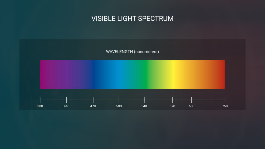
Due to the nature of those wavelengths, they react differently when bouncing around volumes like air or in this case water.
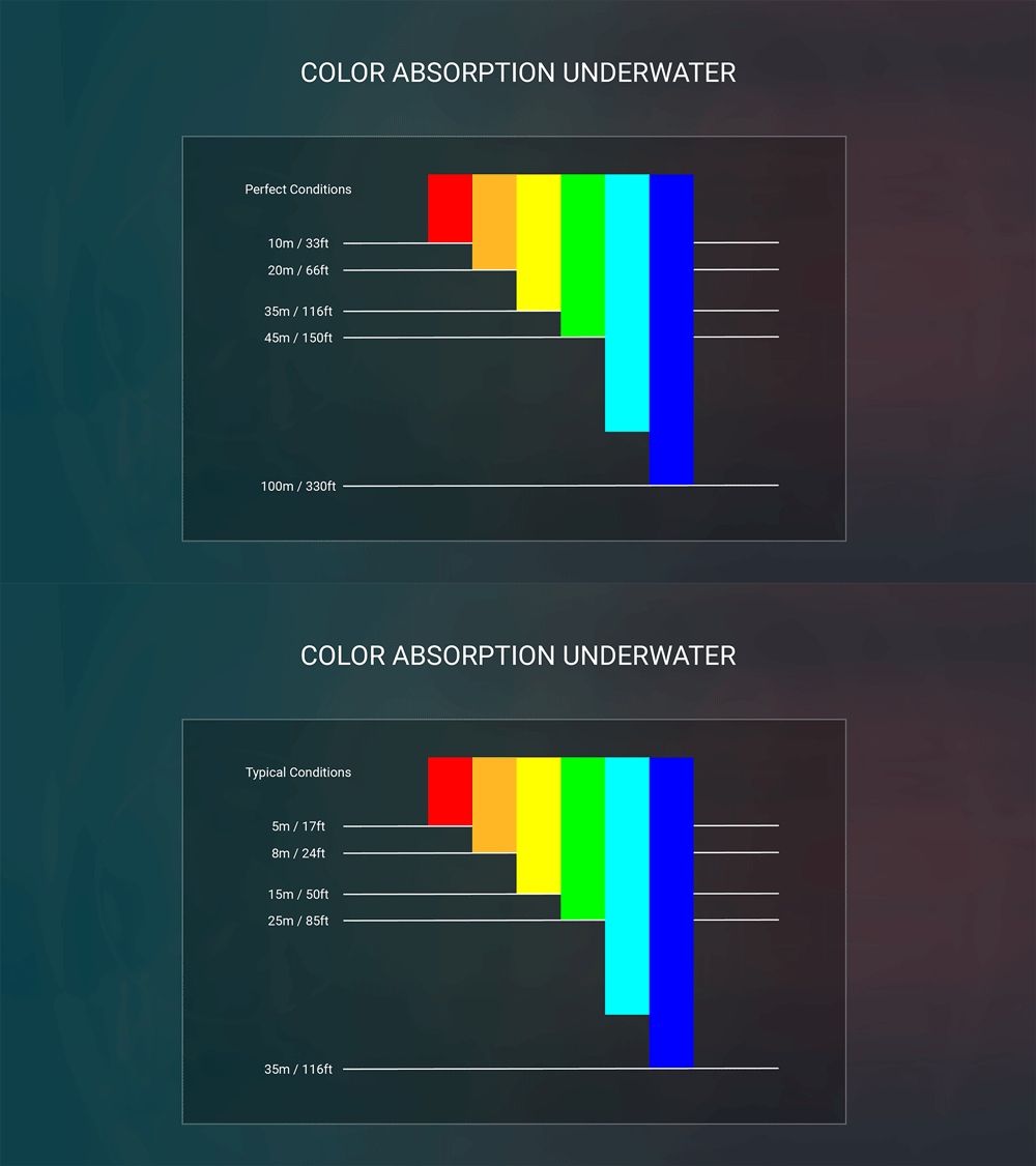
Red light is the first to diminish at a short distance due to its characteristics of being a relatively long wavelength. After that the wavelengths of orange, yellow and green get absorbed by the molecules and particles within the water. Blue, due to its very short wavelength, manages to make its way through for quite a bit longer. So you can already see why the last of an object you can make out underwater is blue-ish.
Now how can we mimic that behavior and maintain a flexible control over the different colors based on distance? Conventional compositing methods will not help us to achieve this look.
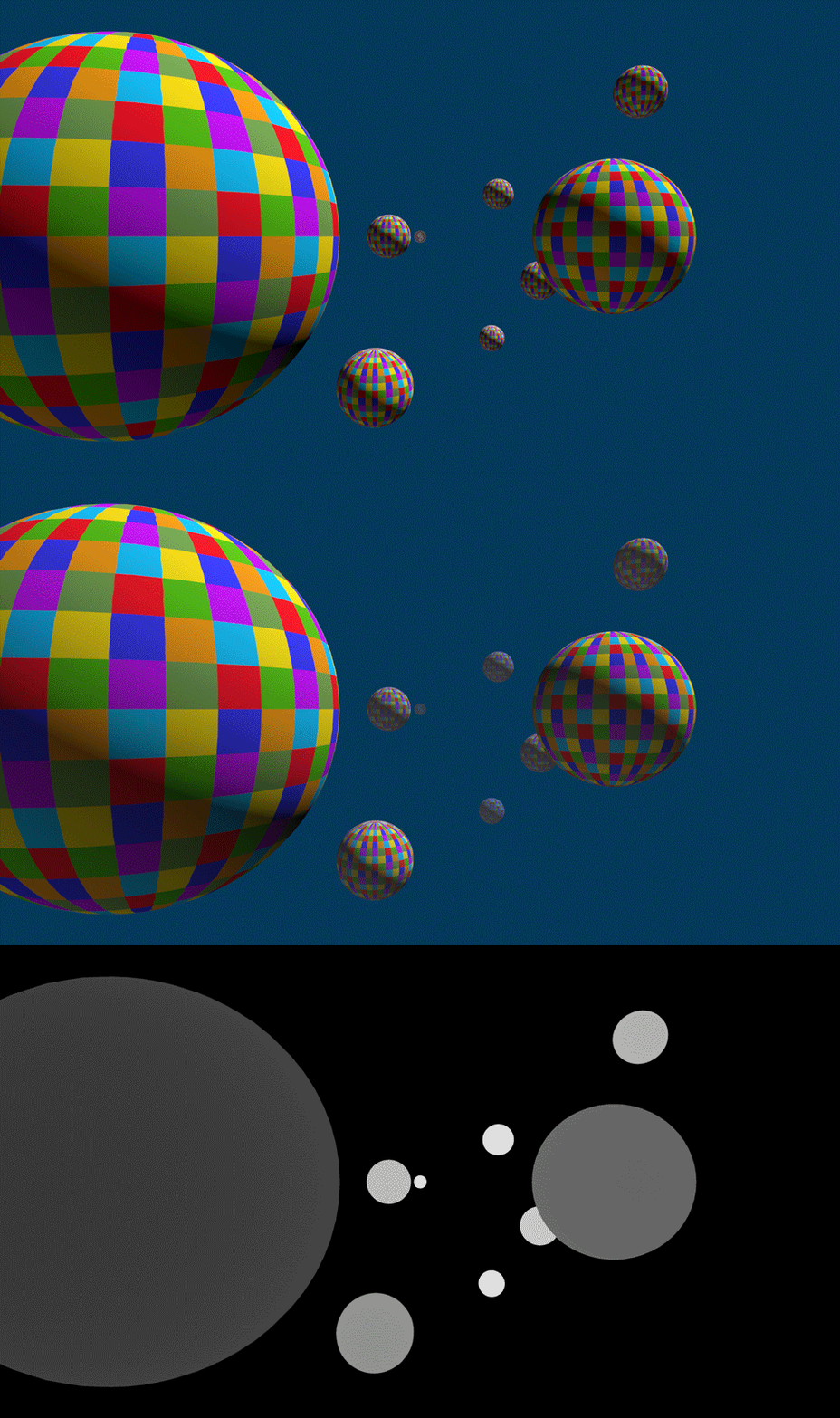
We can also not mimic the selective loss of color at certain levels of depth.
Now how can we imitate that behavior and maintain flexible control over the different colors based on distance?
First of all, we can make use of our 3 color channels: Red, Green and Blue. Then we need to break the linear restriction a normalized mask input gives us. Rather than working with a straight line, we want to define a curve for each of those channels.
I’ll show you a way of having much more control. The tool that makes this possible is the ColorLookup node.
Option 1: ColorLookup Node
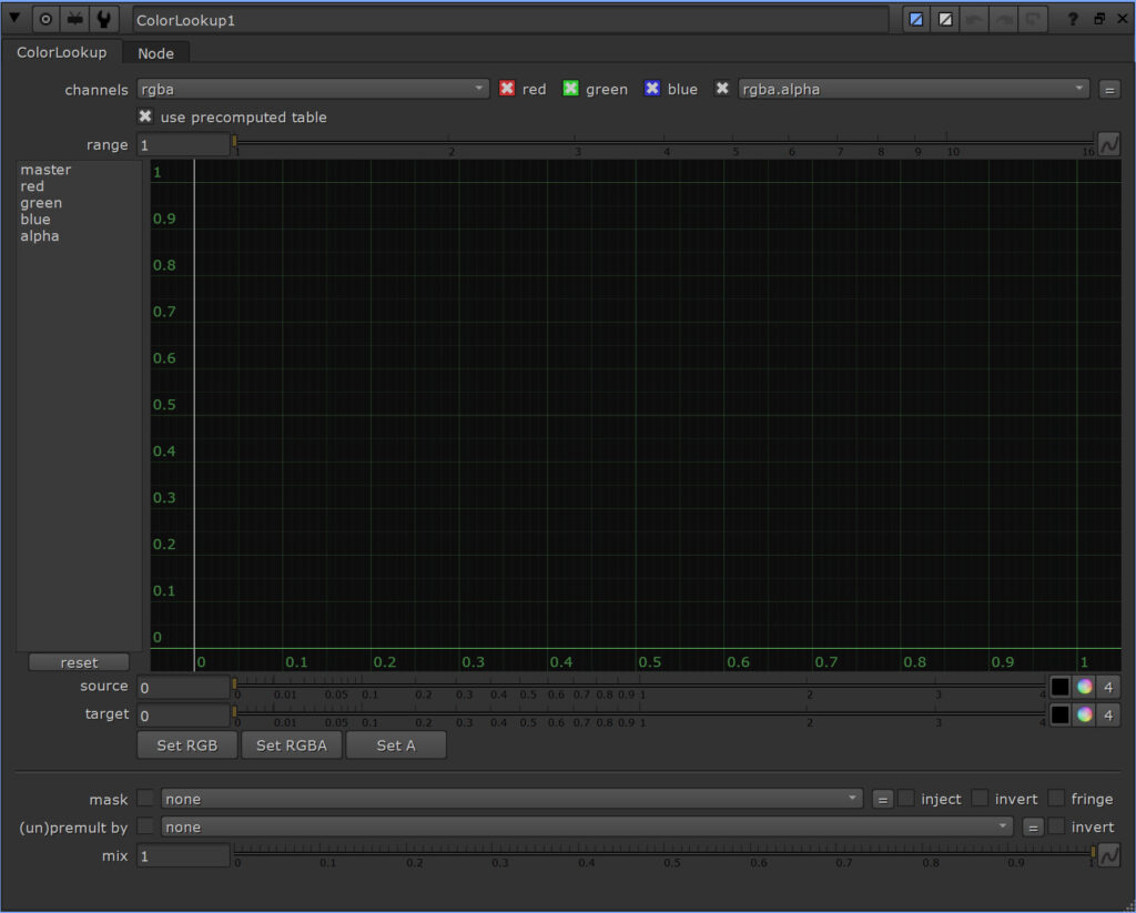
The horizontal x axis represents the original, incoming values while the vertical y axis represents the new value that will come out of the node.
We can add as many points to a curve as we like and adjust the tangents.
In a lot of cases we use the node to adjust the color by changing black and white levels or the gamma. We will learn to use it in a completely different way now by using its capability of being a simple lookup table – so it can do some calculations for us. It will only be used as a processing unit, but we will not use the actual output of the node.
Based on our color depth chart, I want red to fully lose its color at 5 meters – so I define the curve for the red channel based on that. I set a point with the y value of 1 at the x value of 0.
This means that at a depth of 0 we will have full visibility of the color. I set a second point at the x value of 5 – with y being 0. This means that a depth of 5 will have zero visibility of that color. Everything in-between will behave in a linear way.
I do the same for the green channel with 25 and blue with 35 meters.

Now I can use an Expression node to gather the color visibility for every incoming pixel by looking up their y value based on their depth value.
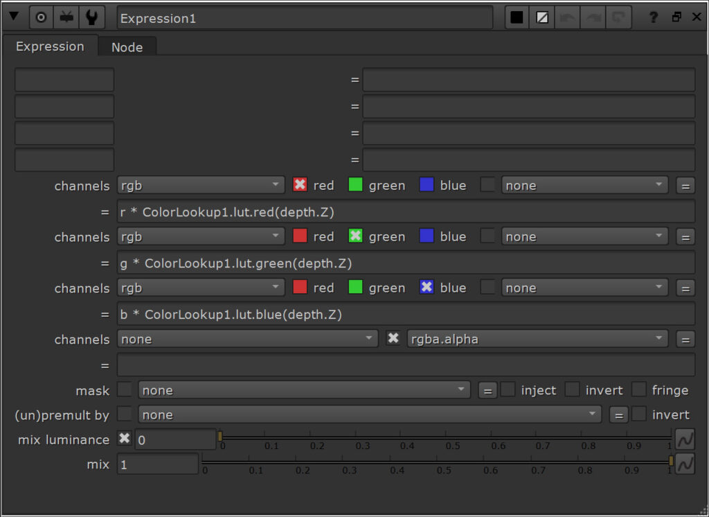
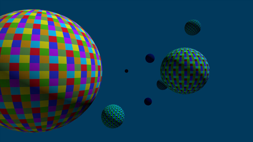
We can also use more than 3 curves to help us with our look. Let’s say I also want to introduce some haze based on depth. I could use the master curve to define those values. In my expression node I assign this curve to a variable first – just to avoid having the actual expression look too complicated. I simply add this variable – meaning that everything at a depth of 0 gets an added value of 0 while everything at a depth of 50 gets an added value of 0.01.
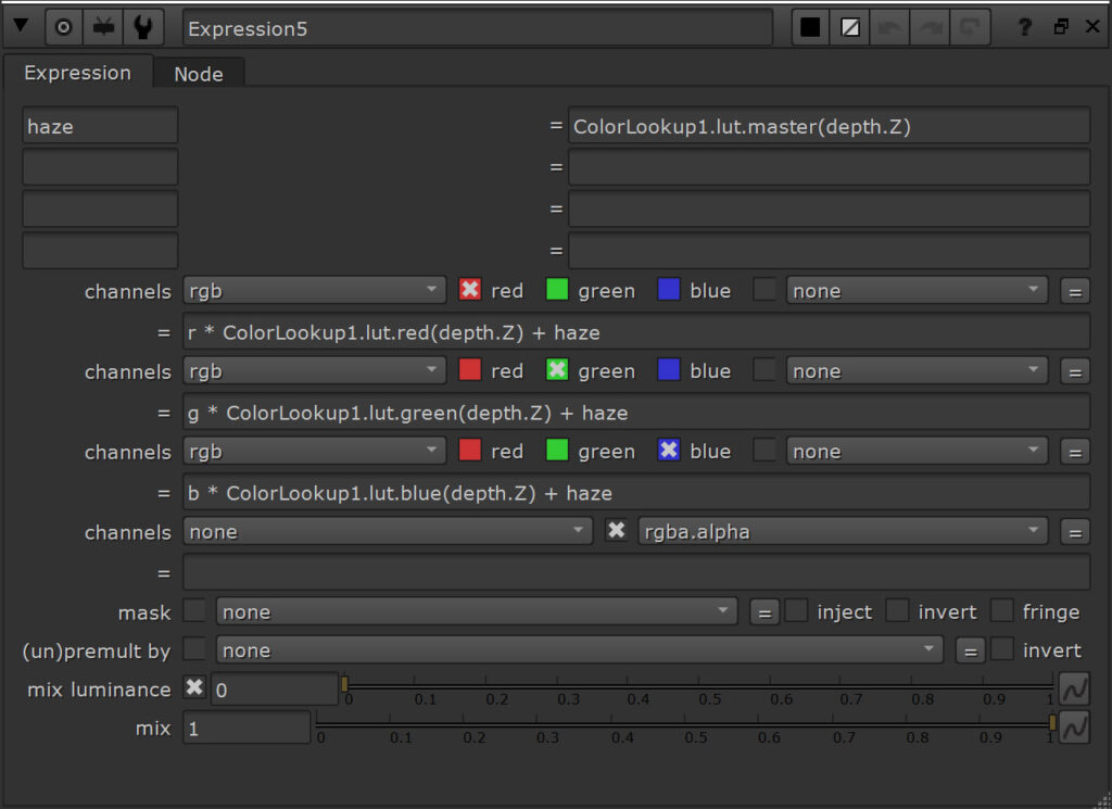
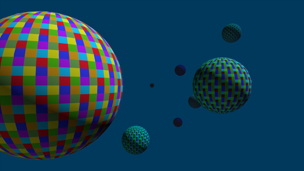
That’s all cool – but with this approach we only really have control over red, green and blue. So let’s leave this example behind and bring our approach to a whole new level.
Option 2: HueCorrect Node
I don’t want to be restricted to the RGB channels, so in addition to knowing the depth value of every pixel, I also wanna know the hue.
By assigning a curve to the table of the HueCorrect instead of the ColorLookup node, we can define maximum depth values for every hue. The plan is to determine the hue of every pixel of our image, find it in the table, determine the maximum depth value for the color to be visible and compare it to the actual depth value to see where we are in that range.
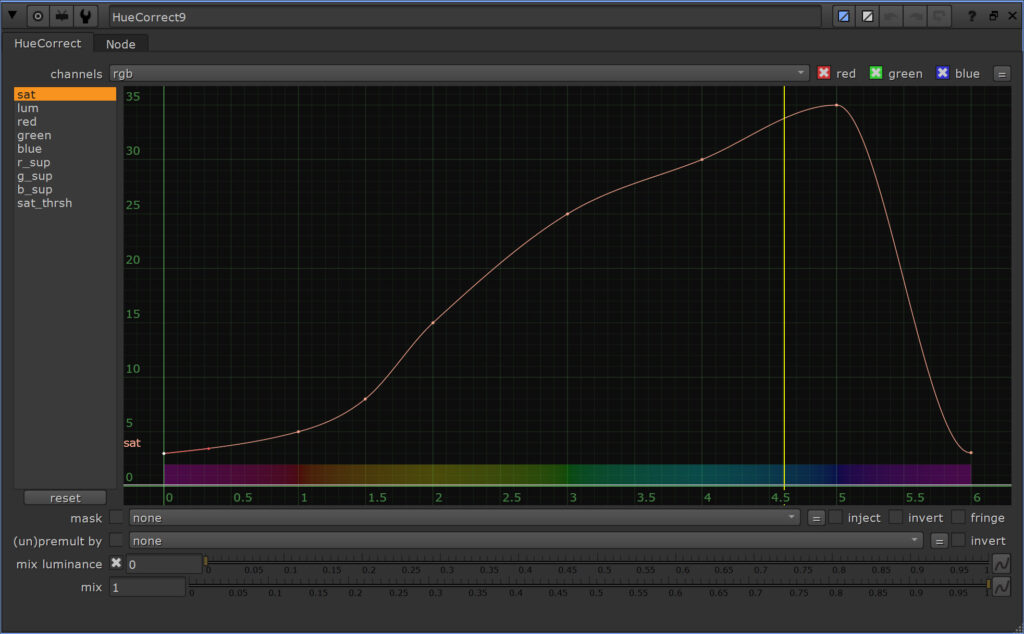
Then we can remove the color from this pixel the closer its depth position is to the maximum depth value. But how do I find the hue values of my image?
I really recommend watching my YouTube episode (or reading the blog post about it) about the HueCorrect node since it includes me going through that topic in depth.
Hue values can be displayed or measured in different formats and ranges – it could be a circle in degrees, in a range between 0 and 1 or as we can see in case of the HueCorrect node, a range between 0 and 6.
If we use a Colorspace node for conversion from RGB to HSL for example – which is Hue, Saturation and Lightness – Hue values are being mapped into our red channel. The range is set between 0 and 1 though.
I will work in this space to reduce the lightness (which is stored in the Blue channel) – but in order to generate a mask for this, I will need a second pipe that converts our RGB image into hues in a 0-6 range.
Expression Setup to convert RGB to Hue values
I use the following expression setup to do this:
# First I define 2 important variables in the upper section of the Expression node.

min_value = min(r, g, b)
max_value = max(r, g, b)

# Then I'll set the actual expression for the red channel (it could be any other channel).

r >= g && r >= b ? (g-b) / (max_value - min_value) : g >= r && g >= b ? 2.0 + (b-r) / (max_value - min_value) : 4.0 + (r-g) / (max_value - min_value)
I add another Expression node to avoid nan values:
isnan(r) ? 0 : rThe hue values are offset from how they are distributed in the HueCorrect node, so I add an Expression node to compensate for that:
r != 0 ? r + 1 : 0Finally, I add one more Expression node to offset negative values:
r < 0 ? r + 6 : rOf course we could make all of this work in one Expression node, but this way it maintains a better readability and we can clearly see the different steps.
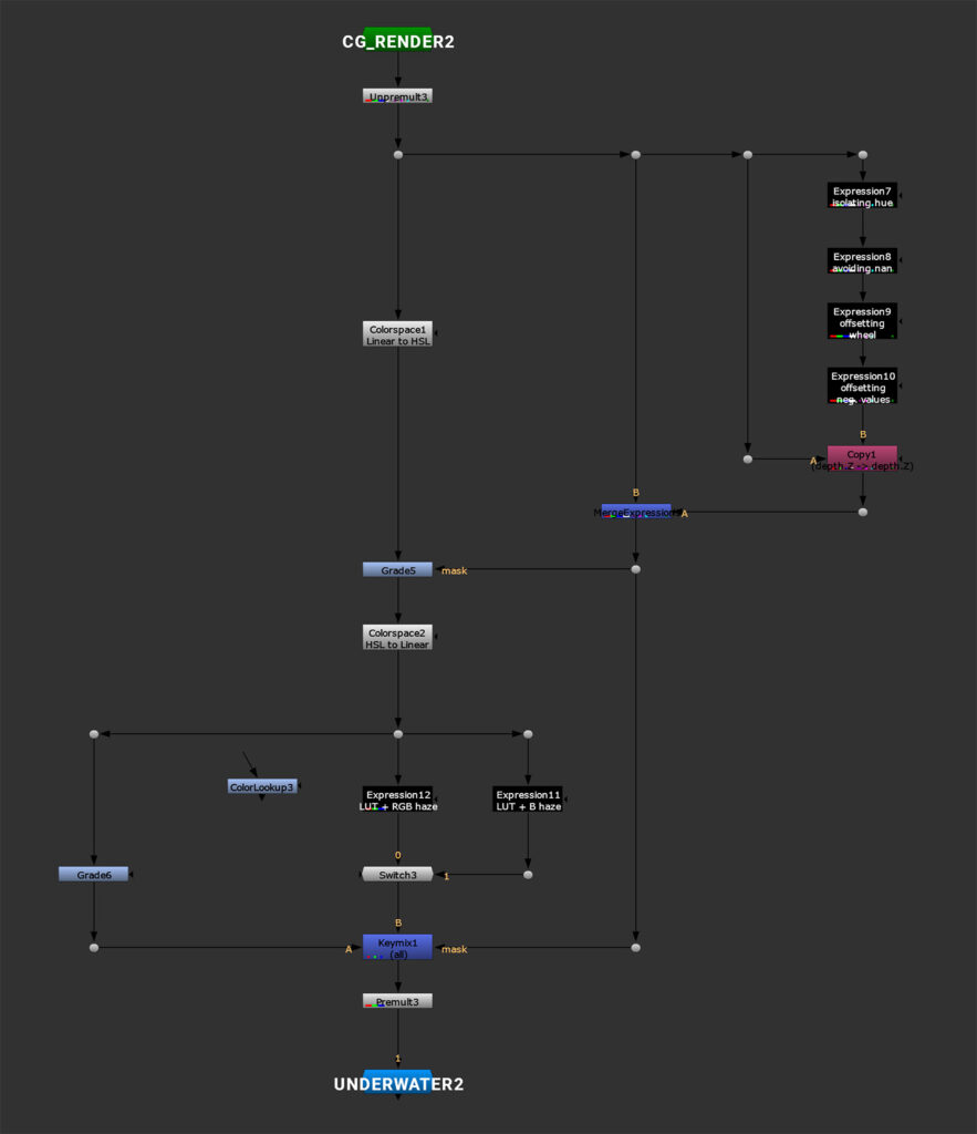
I also shuffle in the depth pass from my original image. For better visibility I use a MergeExpression node now.
The original image is coming in via the B input, while the expression generated hue pass plus the shuffled in depth pass go in via the A input.
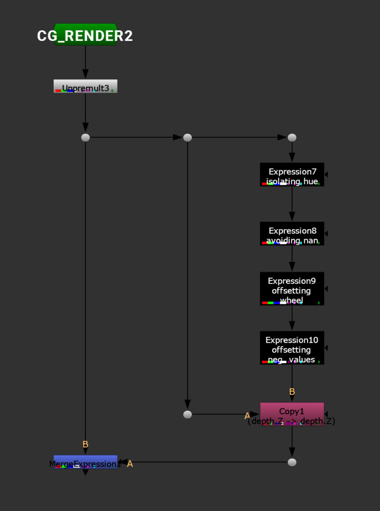
Let’s define some variables.
I want to know the maximum depth (maxDepth) value of the incoming hue – so I need the y value of our curve for the incoming hue or x value.
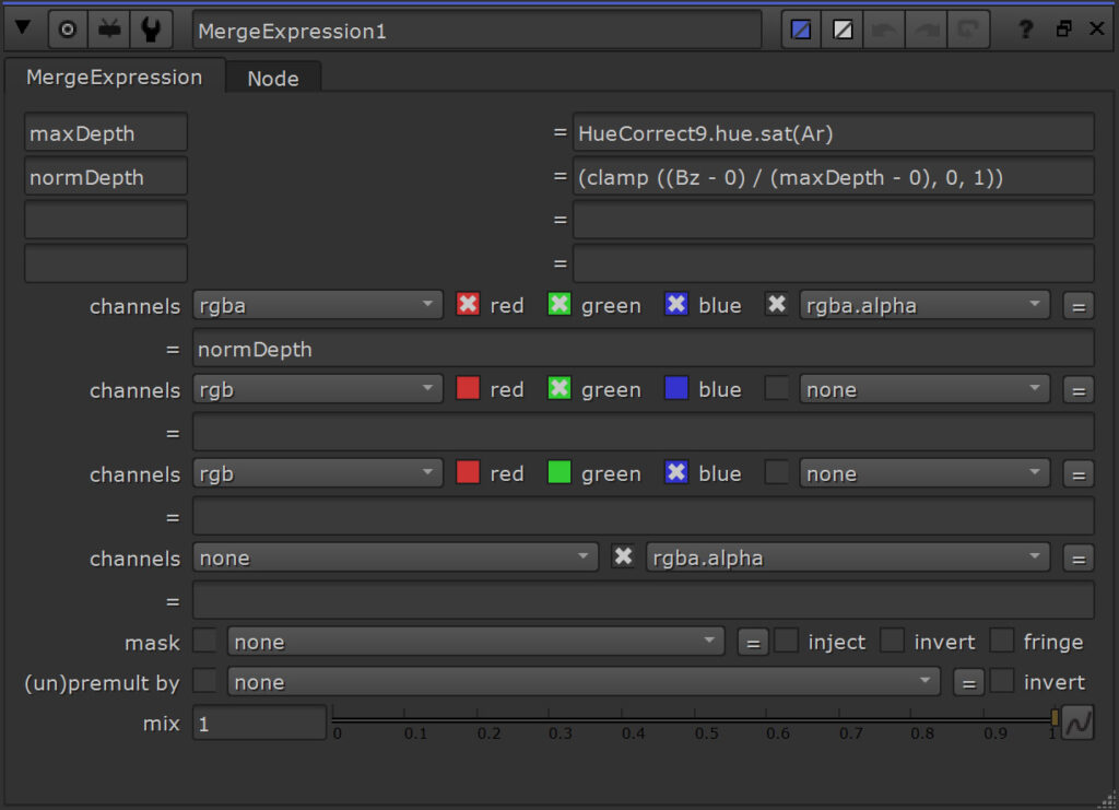
Then I want to normalize this depth range – from 0 to the maximum depth value into a range of 0 and 1.
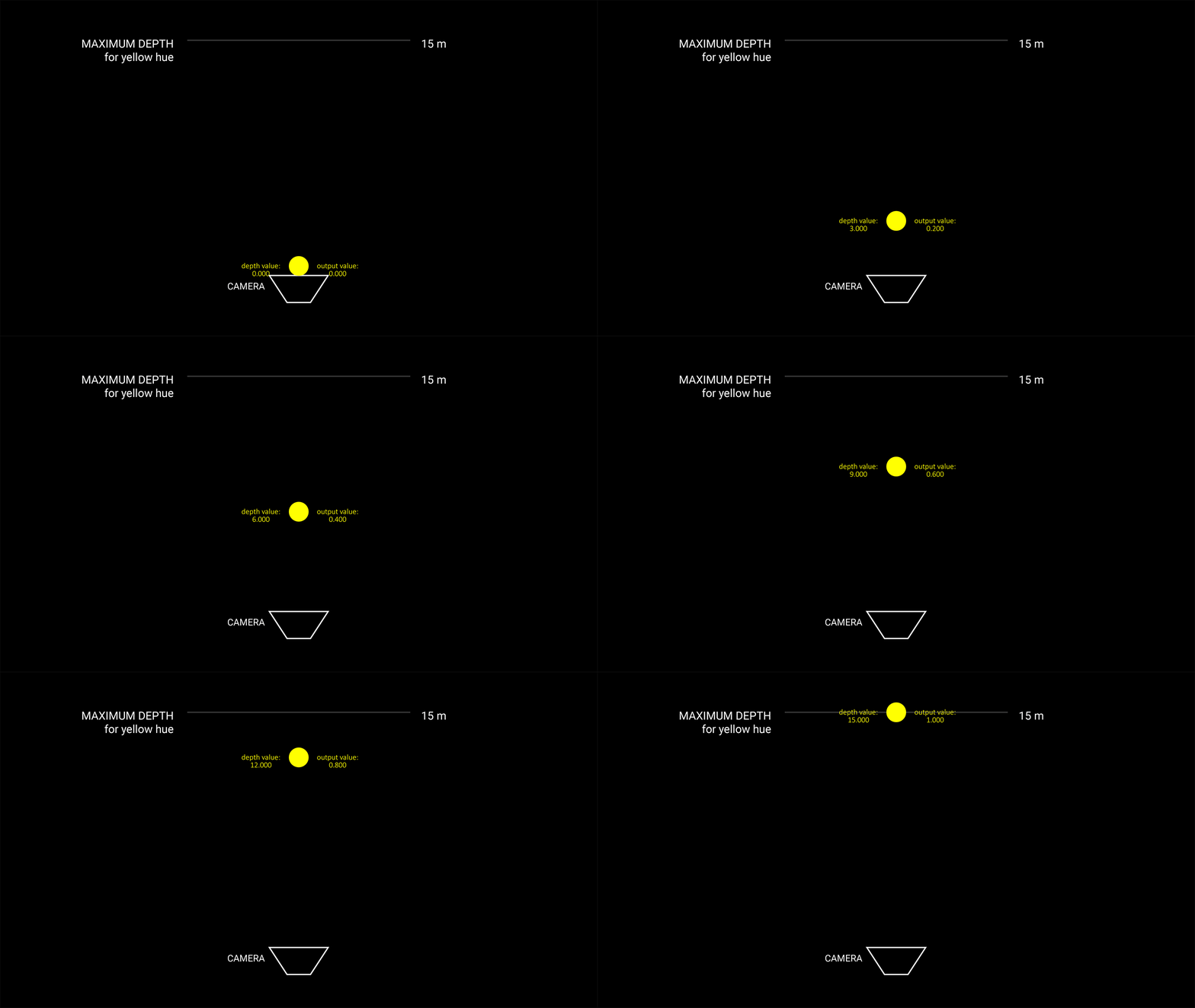
The number will increase in a linear way while the pixel is moving towards its maximum depth – with 1 being the output right at that maximum value.
I set up another variable to create a normalized version of the range between 0 and the maximum depth value for the corresponding pixel (normDepth).
By knowing the formula for normalization, I use the depth channel z of my B input as the incoming value, our maxDepth variable as the max value and 0 as the min value.
(Bz - 0) / (maxDepth - 0)I’ve nested the normalization inside a clamp expression:
clamp( (Bz - 0) / (maxDepth - 0), 0, 1 )I clamp the values at 0 and 1. When our actual pixel depth value goes beyond its maximum value the number doesn’t increase beyond 1 that way. The reason is that I want to use the output as a mask to desaturate the pixel.
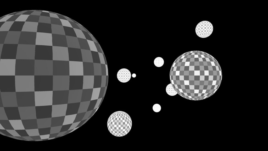
I’m actually not desaturating it per se – I am reducing the lightness of that color value.
I add a Grade node to the main pipe of my image, right after the Colorspace node which I used to convert RGB to HSL.
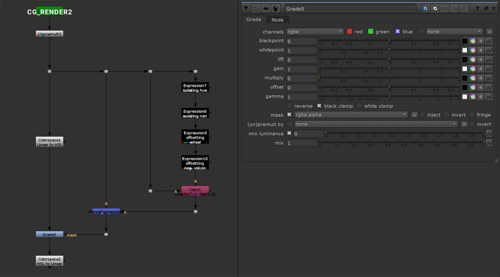
I use the mask that I generated with the MergeExpression node for the mask input and dial down the Gain or Multiply sliders of the Grade node to 0.
Bright areas of our mask – meaning pixels that are close or at their maximum depth will get their lightness reduced.
After that I’m converting the image back to RGB – and the colors disappear according to the depth values I defined.
There are different ways of applying an overall depth haze again – as we’ve seen in the ColorLookup approach before. I’m using another ColorLookup node for that – so I’m free to edit the curve for different depth values individually.
It could be applied to all the channels or maybe just the blue channel, since that’s the color that would be visible the last. Also, I’m adding a bit of a blue lift to the colors that are starting to fade off – reusing the mask we generated with the MergeExpression.
Let’s compare the outputs:
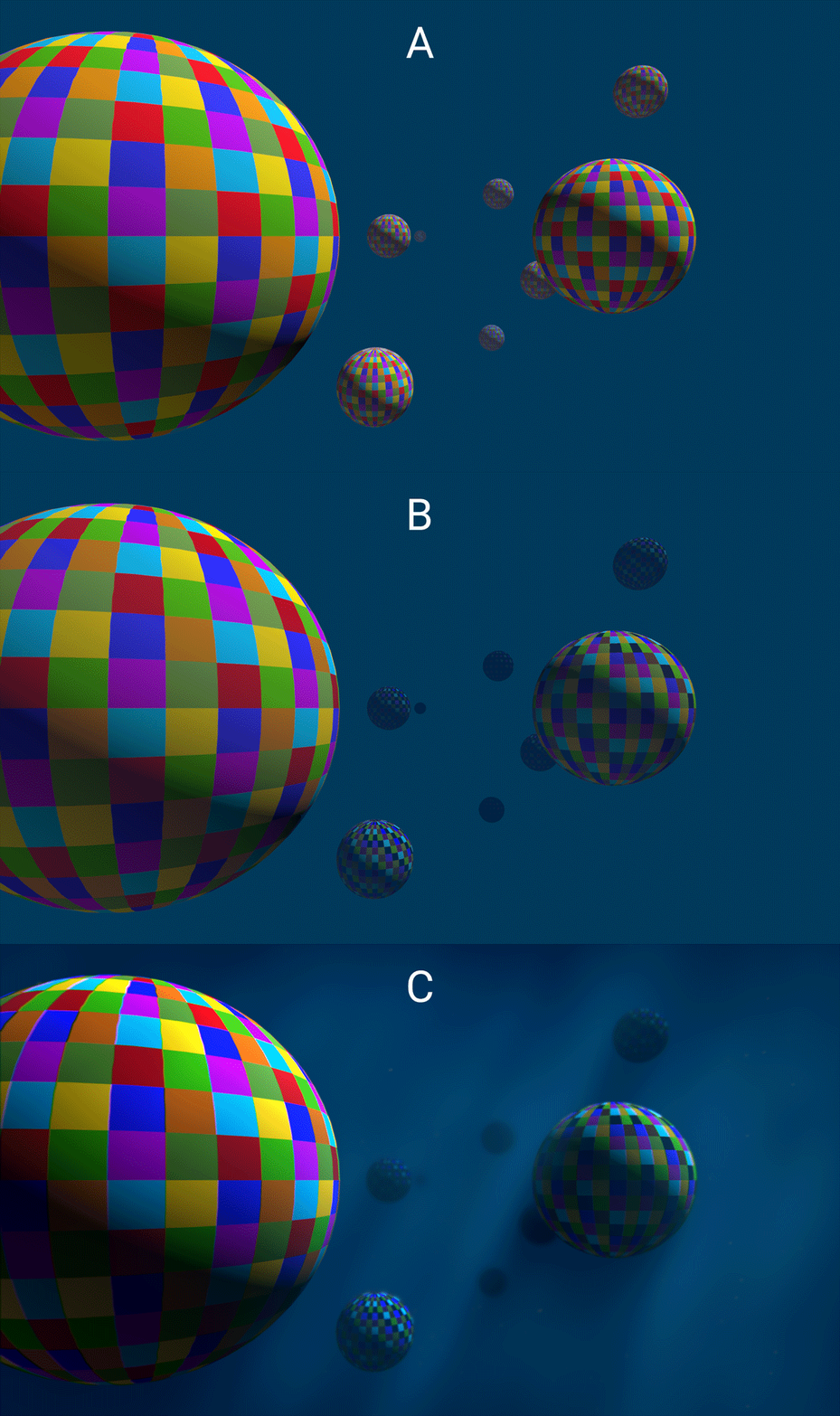
(B) Hue curve approach
(C) Hue curve approach with a quick setup of underwater atmos (diffusion, volume rays, particles, chromatic aberration)
Bonus: Customizing Curve Names
As we’ve learned, we can utilize the curves of a ColorLookup node not only for RGBA. Nonetheless we seem to be stuck with those names and it could be a bit misleading if someone else is working with our script.
We can use python to remove and add custom curves with our own naming. With node.knob I can access any knob of this node.
The one we are looking for is called lut – an information we can gather by hovering over the knob. But hovering over the curves also only gives us the knob name “lut”.
Well, the ColorLookup knob is a class on its own, which comes with certain methods we can use. For example, we can delete a curve with the method “delCurve”, followed by the curve name. Curves can be added by the method “addCurve”, followed by a name of our choice.
That can help us with a better read on what we are using this curve actually for.
I hope you enjoyed this little brainstorming session and find your own fun ways to utilize curves for example for very controlled depth treatment.
Please feel free to watch the video for more detailed and in-depth information.
You can download the Nuke script that I set up here: UnderwaterLook
