I’m releasing this blog post exactly one year after my first published YouTube video. For that reason it will be a fusion of both my show formats, Nuke Timeout and Unleash The Node.
We’ll focus on one node but keep it short and simple – Espresso Style. Today it’s all about the Hue/Correct Node.
I always found that all the available treatment options can be quite overwhelming and hard to understand what the difference between them is. For example: If I want to reduce some green in my image – do I choose the saturation, green or green suppress option? We will also learn in which order all the different operations are getting applied.
After reading this post you will definitely have a good understanding of what’s going on under the hood and it will help you to make the right choice.
I would like to thank The Foundry, all of my supporters, followers and newsletter subscribers – as well as everyone who reached out with feedback – good and bad. Thank you for making this past year an exciting and fruitful one.
Background Knowledge
The first thing we have to talk about is what all the available options have in common – and it’s this graph:
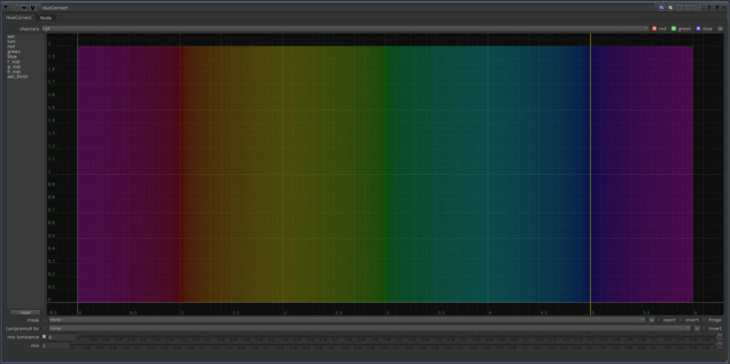
We know it from another node in Nuke – the HueKeyer. We also know the concept of a color wheel. It’s an abstract, circular arrangement of colors organized by their chromatic relationship to another.
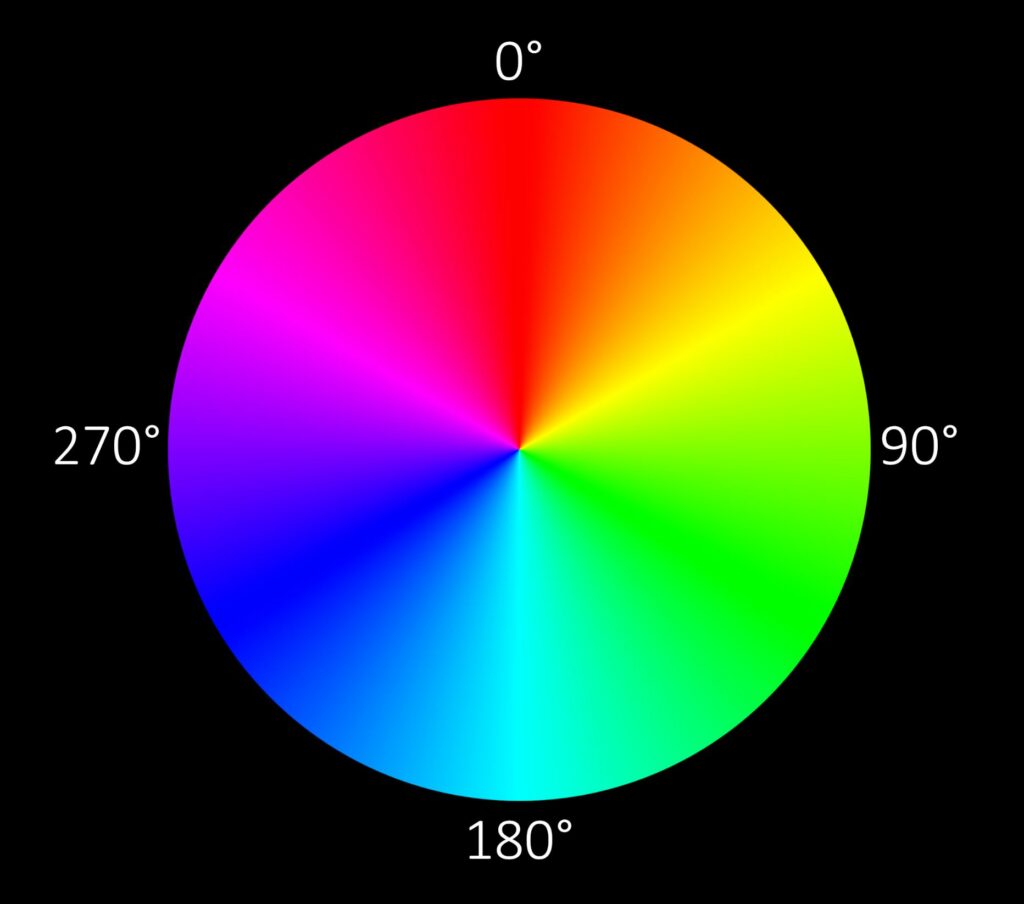
In math classes we learned that a circle has 360 degrees. So we can describe or find a specific color or hue by its degree coordinate if you will. But how do we get the hue value of specific areas or pixels of our image? After all, we usually deal with our 3 channels – red, green and blue. Each of them are combinations of hue, saturation and luminance. Let’s have a look at the mathematical formula for the conversion from color channels to hue:
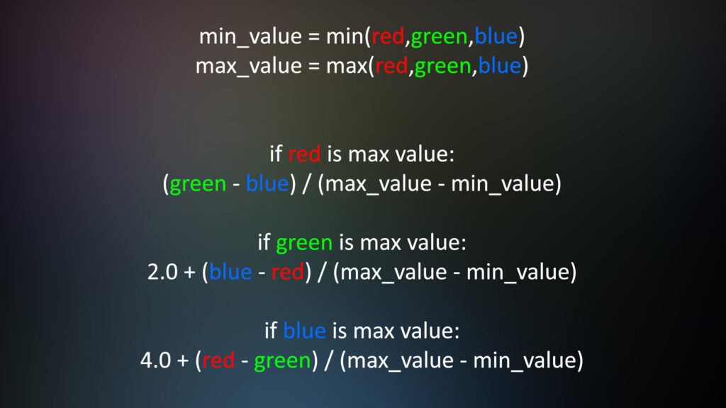
First of all we need 2 important components: the darkest and the brightest value of every pixel. Then we have to compare the different channels with each other.
You can see that every formula is offset by 2 from the others. That way we are able to fit in all of our hue values between the range of 0 and 6.
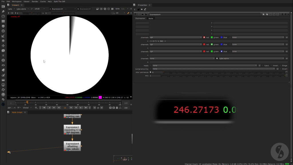
We use all this in an Expression node by using the TCL syntax.
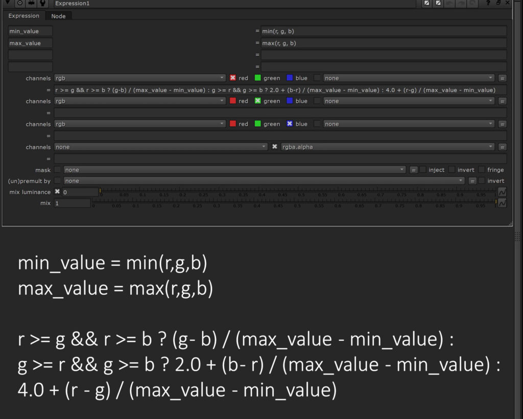
This might give us some nan values, which we will simply set to 0.
isnan(r) ? 0 : rWe have to multiply the resulting values by 60 in order to convert it to degrees on a color circle.
r * 60If we now have negative values, we need to offset them by 360.
r < 0 ? r + 360 : rNow every value sits right at its correct position in the color circle. Instead of sampling our red, green and blue pixel values, we are now able to see the actual degree of our pixels on the hue wheel.
Obviously, we can simplify all this by using only one Expression node, but I just wanted to show you step by step how this conversion works. Also, there is an easier way in Nuke to extract or isolate hue values – by using the Colorspace node. We can either set the output to HSL or HSV – interesting for us today is only the first channel and it’s the same for both options. Looking at the values though, we seem to only find values between 0 and 1.
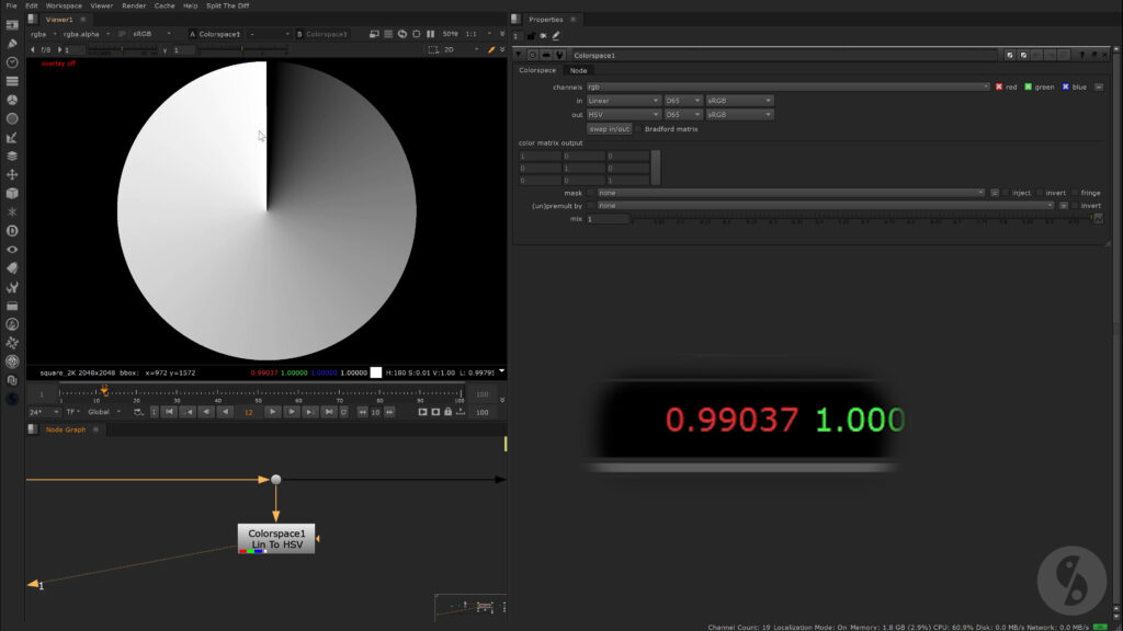
Where did our 360 degrees go? The RGB to hue conversion that happens in the Colorspace node outputs normalized values though – so everything sits between 0 and 1. In order to get to that result we simply divide our values from before by the maximum amount of degrees we have – which is 360.
r / 360That will keep a value of 0 at 0 and set a value of 360 right to 1. So nothing gets higher than that.
Alternatively we can skip the step of converting it from the 0 to 6 range up to 360 and instead we divide it by 6 to normalize it. Instead of offsetting negative values by 360, we now only need to offset them by 1 – since our 360 degree range is compressed into a range of 0 and 1.
r / 6

r < 0 ? r + 1 : r
I also have to add that I had to convert the input to sRGB before going through our formula, in order to match the output of the Colorspace node.
Now it gets a tiny bit more confusing. In Nuke’s HueKeyer we get a linear mapping of hues from left to right, ranging from 0 to 6. So there is no need to multiply our formula values by 60 – every unit stands for 60 degrees. 6 times 60 is 360.
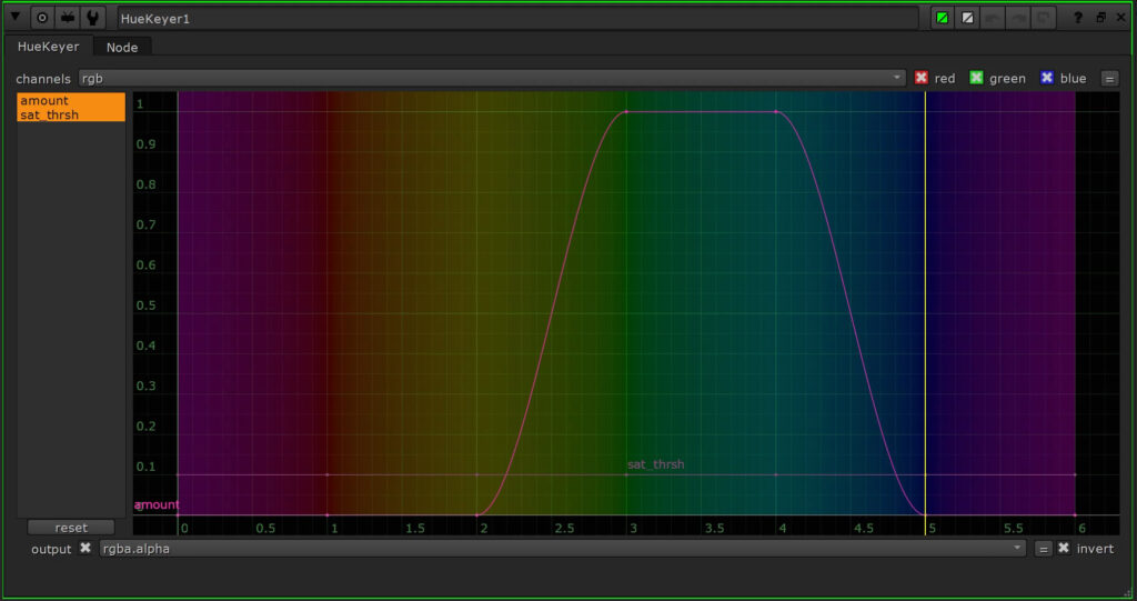
We have to make a different adjustment though. For some reason the hue ramp in the HueKeyer node is offset by 60 degrees from the color wheel. Since every unit represents 60 degrees, we have to add 1 to our values – but we leave 0 untouched. Now everything sits in the right space.
r != 0 ? r + 1 : 0To sum it up:
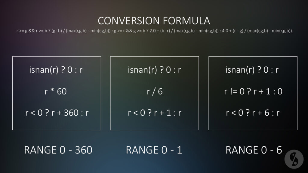
The base of it all is the conversion formula. In all cases we want to get rid of nan values.
Since the conversion will squeeze our hue values into 6 units, we can then decide if we want to stay in that range to match what the HueKeyer is using. We only need to offset all the values (except 0) by 1. This is what we can see on the right side of this graphic.
On the left we can see what we have to do in order to stretch all the values to 360 degrees. We simply multiply the 6 units that the conversion formula outputs by 60. 6 times 60 equals 360.
The example in the middle shows us how to normalize the 6 units into a range of 0 and 1 – by simply dividing by 6.
For all the 3 options we then have to take care that negative values will be offset into positive space while maintaining the respective range.
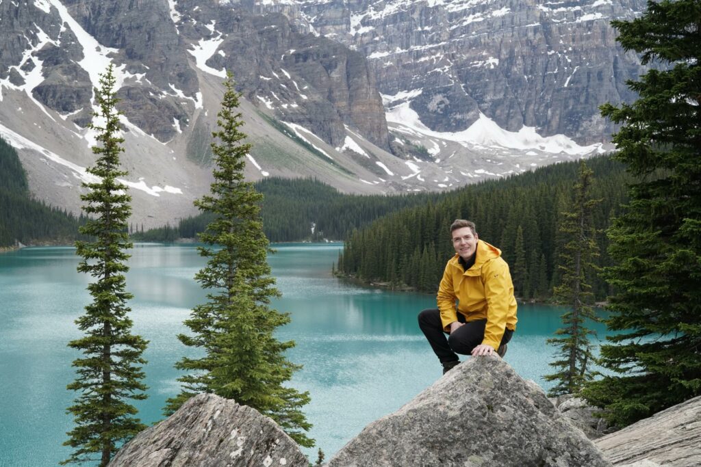
Now that we clarified what a hue is and how to get to it, let’s talk about the HueKeyer node. It enables you to pick specific hue values or actually ranges and create an alpha for them. That way you can use it as a mask for other operations – for example if we want to desaturate this range of hue values.
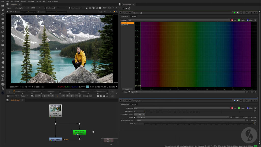
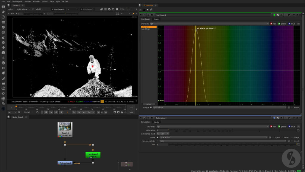
The saturation threshold value takes a look at the saturation of our image and helps you to isolate areas even more. We can see that not only the jacket, but also the face got affected quite a bit. Luckily it’s less saturated than the jacket. If we increase the saturation threshold above the saturation value of this area, it will drop out of our selection. That way we can preserve more of the original saturation.
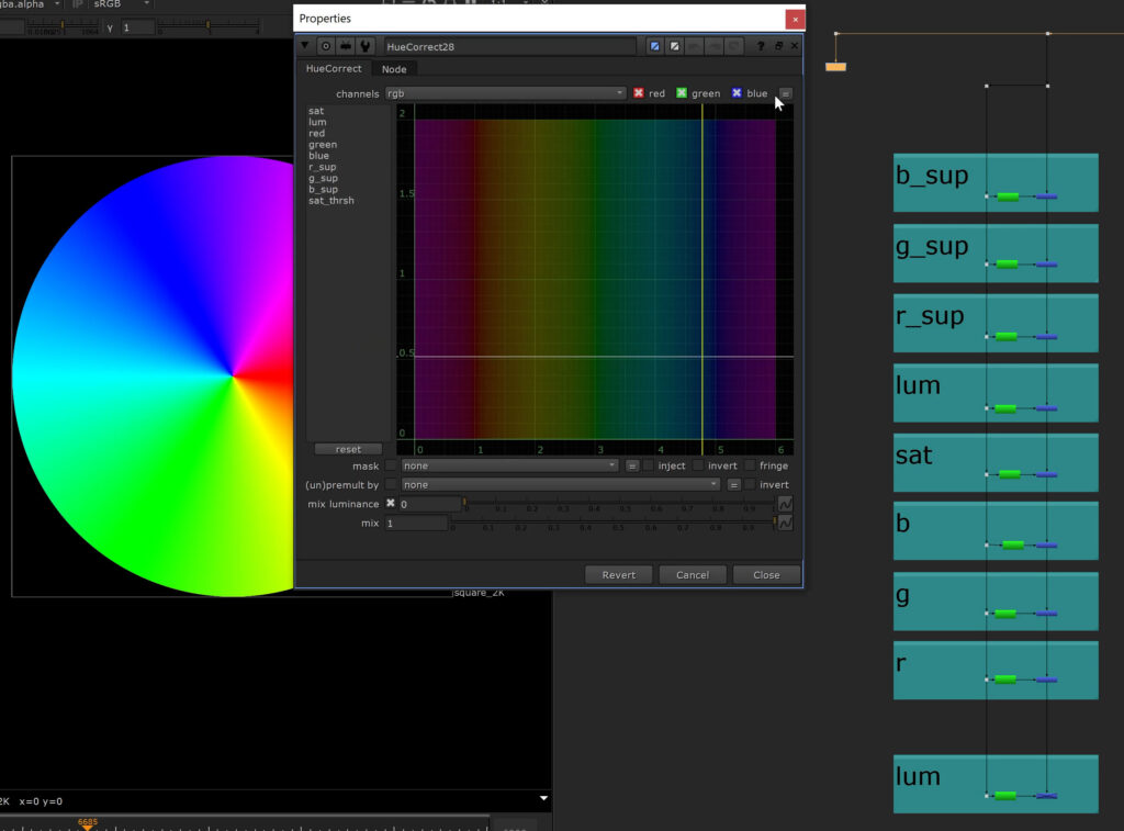
Deconstructing HueCorrect
Ok, we got all the background knowledge out of the way. If you’re wondering why I talked anout all this.
When deconstructing the HueCorrect node, we will notice that all the different operations available can be broken down as:
Number 1 – applying a mathematical formula and
Number 2 – applying it through an alpha created by the Hue ranges we define with our curves;
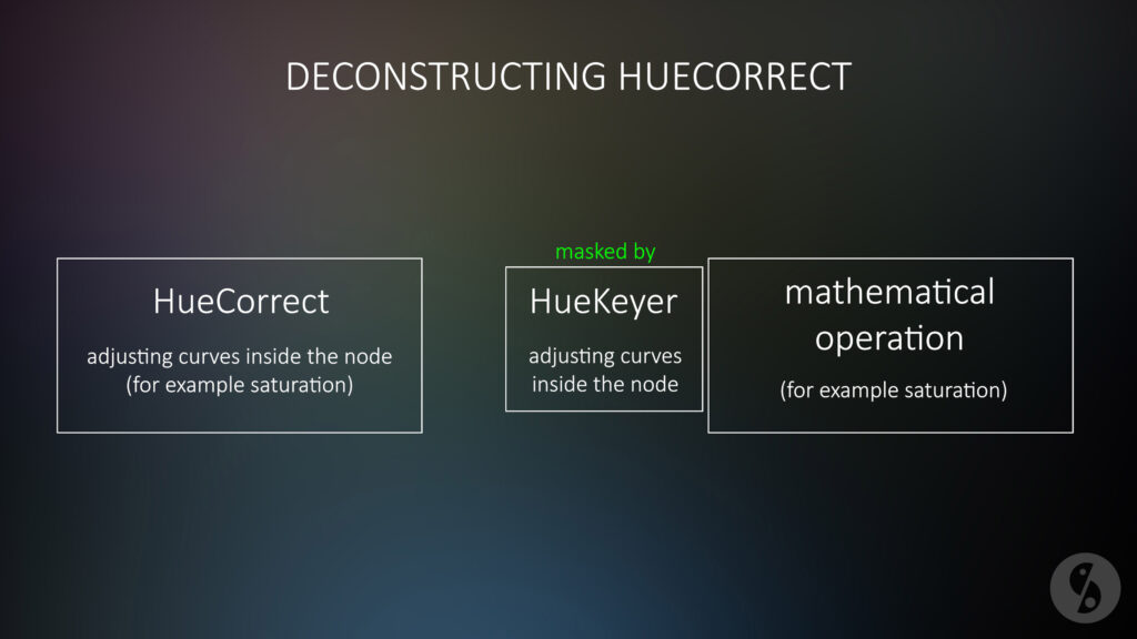
You’ll see in a minute what I mean. Let’s go over all the different treatment options from top to bottom.
We start with Saturation. Under the hood, increasing or reducing saturation can be done in multiple ways with different formulas.
One of the most common approaches is to use the rec709 luminance math. Since our eyes perceive certain wavelengths or colors brighter than others, although they might have the same contribution to an image, this formula helps us to simulate that.
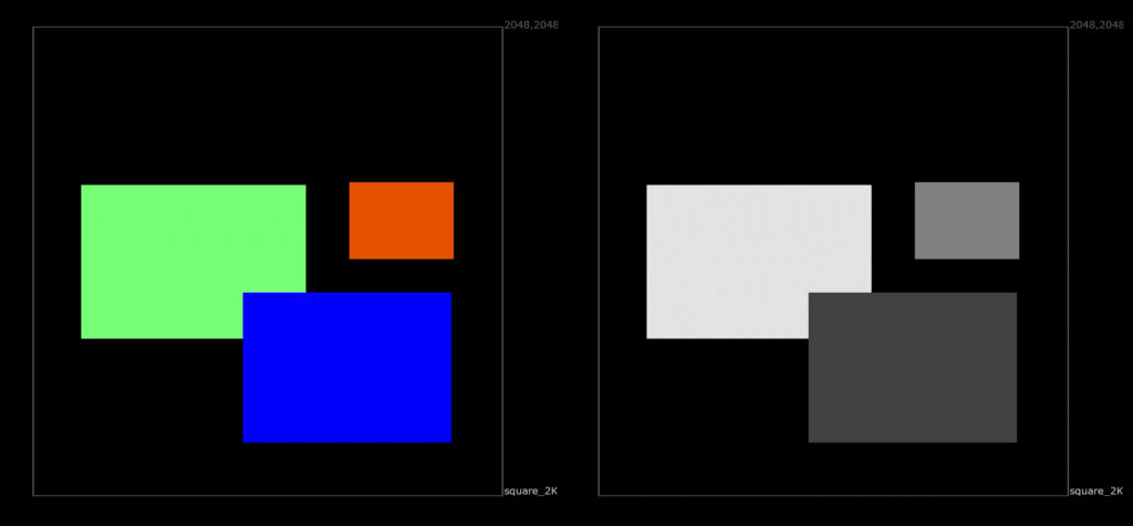
If we look at this image for example, green clearly pops out brightness wise, although we have a very strong blue presence too. If we convert an image to it’s grayscale representation, we want to make sure that this are still looks the brightest. In the red and blue channels, this area is rather dark, so we should not simply create an average of all three channels – we need to prioritize green. Out of our 3 channels, our eyes are the least sensitive to blue.
That’s why the International Telecommunication Union came up with the following formula:
BT.709 → Luminance = Red*0.2126 + Green*0.7152 + Blue*0.0722 - with those three coefficients adding up to 1
The HueCorrect Saturation operation uses a variation of this called BT.709-1:
Luminance = Red*0.2125 + Green*0.7154 + Blue*0.0721
To increase or decrease saturation you use a function called Linear Interpolation or “Lerp”:
Final pixel = alpha * color1 + (1.0 - alpha) * color2
Color1 in this case is the normal color of our image, while Color2 is the fully desaturated version of it. I will use a MergeExpression node in order to use this calculation for every one of our 3 channels.
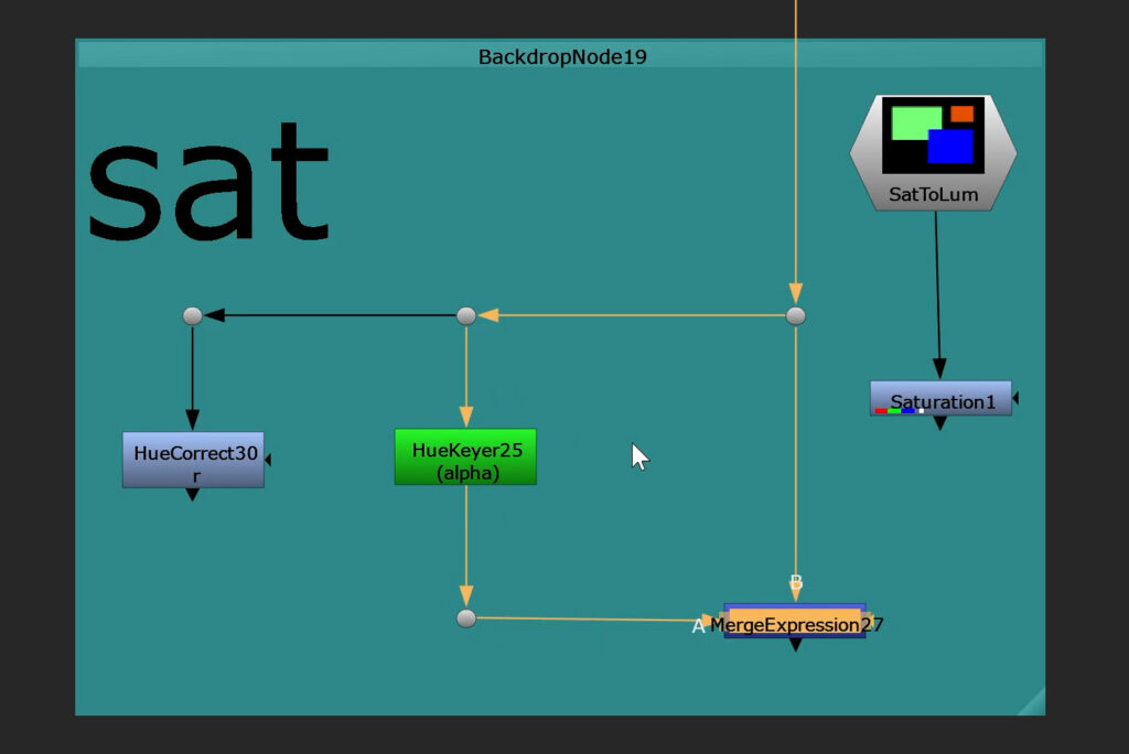
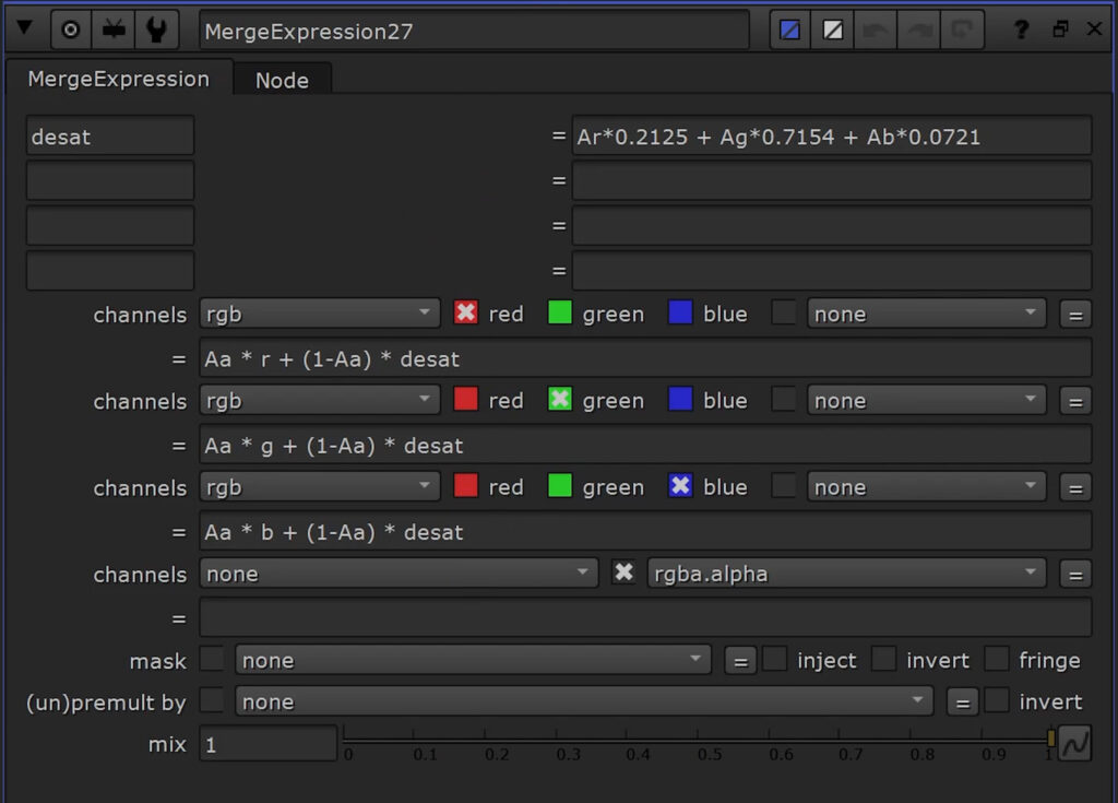
We already talked about how to desaturate an image. I store this in a variable called desat, so we don’t have to type it out for every channel. And now I use our Lerp function. Upperscale A, lowerscale A means, I’m using the alpha channel of input A. Color1 in this case is our respective color channel.
Let’s randomly adjust the curve and see what happens. Certain hue areas experience a decrease in saturation, others stay the same.
If I would use a fully white alpha now as input A, our image would end up fully desaturated. Instead, I will use a HueKeyer and use the same values on our curve that I used for the actual HueCorrect. It matches.
I hope that setup helps a little bit to understand what happens under the hood. Let us go over the next operations and you will see and understand the pattern here.
Next up is luminance.
I choose some random values again – which leads to areas becoming brighter and other areas becoming darker. This is a simple multiplication.
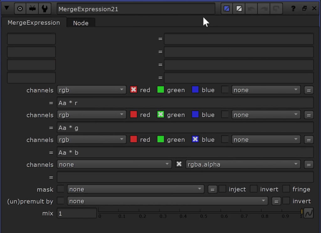
All 3 channels get multiplied with the same value – the incoming alpha channel – from input A in this case. The HueKeyer matches our HueCorrect again and it matches.
The R, G and B operations basically do the same thing – but for one channel at a time only.
The 3 individual operations match their respective deconstructed setups. Of course you could use them in a stack or the channels can be shuffled together – in order to match the HueCorrect node that has all 3 operations combined in one node.
I hope you can understand the pattern now. Under the hood every operation triggers a mathematical formula and then uses our hue curve to generate values to multiply with – to put it simple – the hue curve adjustments create our alpha.
R_sup, g_sup and b_sup use a concept called color suppression.
A common field of usage for it is keying. The green or blue screen might be visible through semi transparent areas like motion blur or the color is just so strong that it bounces around the set and it gets reflected a lot. The color spills over.
We then use the so-called spill suppression – which is basically the same. What it usually does is compare our 3 color channels and based on the algorithm we use it removes or suppresses the chosen color and replaces it with one of the other channels or combinations of it.
There are a few common algorithms out there. Let’s say we want to suppress our green channel.
We have an algorithm called Blue Limit.
g > b ? b : gIt determines where the values in the green channel are higher than the blue channel and if that is the case, the green channel adapts or will be replaced by the value of the blue channel.
There is an algorithm called Red Limit.
g > r ? r : gSome formulas get a bit more complex like Average – which outputs a mix of the red and blue channels.
g > ((r+b)/2) ? ((r+b)/2) : gWe have something called a Double Blue Average…
g > (2*b+r)/3 ? (2*b+r)/3 : g…or Double Red Average.
g > (b+2*r)/3 ? (b+2*r)/3 : gI was playing around with a lot of different algorithms in order to match the one that the HueCorrect Node is using and it seems to be a slightly different version – a combination of formulas.
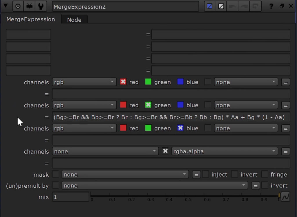
We also have to use our Lerp or Linear Interpolation function again in order to blend the values based on the incoming alpha channel.
If I compare the outputs between the individual HueCorrects and our Under The Hood setups, it seems to do the job.
Here is the adjusted formula for the blue channel…
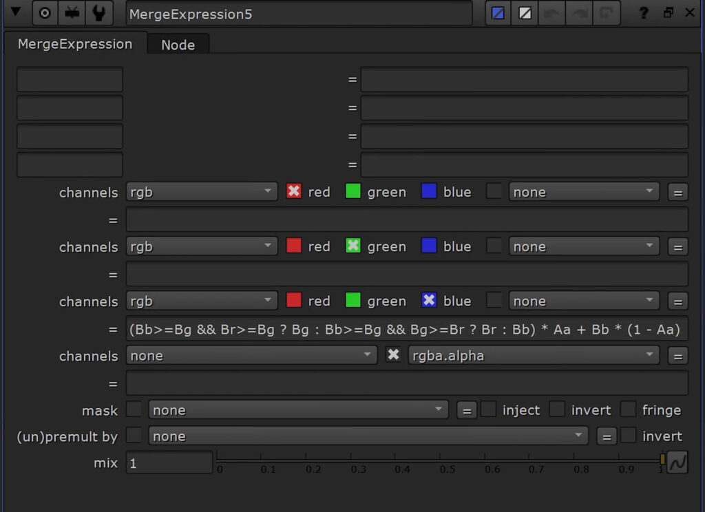
…and here for the red channel.
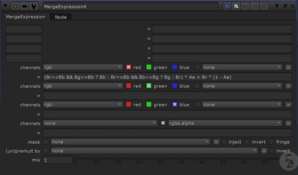
Alright, one last thing.
I played around with the order of operations to see how the HueCorrect node gets processed internally. It seems like it starts with color suppression operations, followed by the saturation and it ends with the individual color channel multiplications. I was able to place the luminance operation before the saturation operation, but it’s also possible to use it at the end instead, since it is just a simple multiplication.
I added up all of our individual operations into that single HueCorrect and it matches that specific order.
Practice
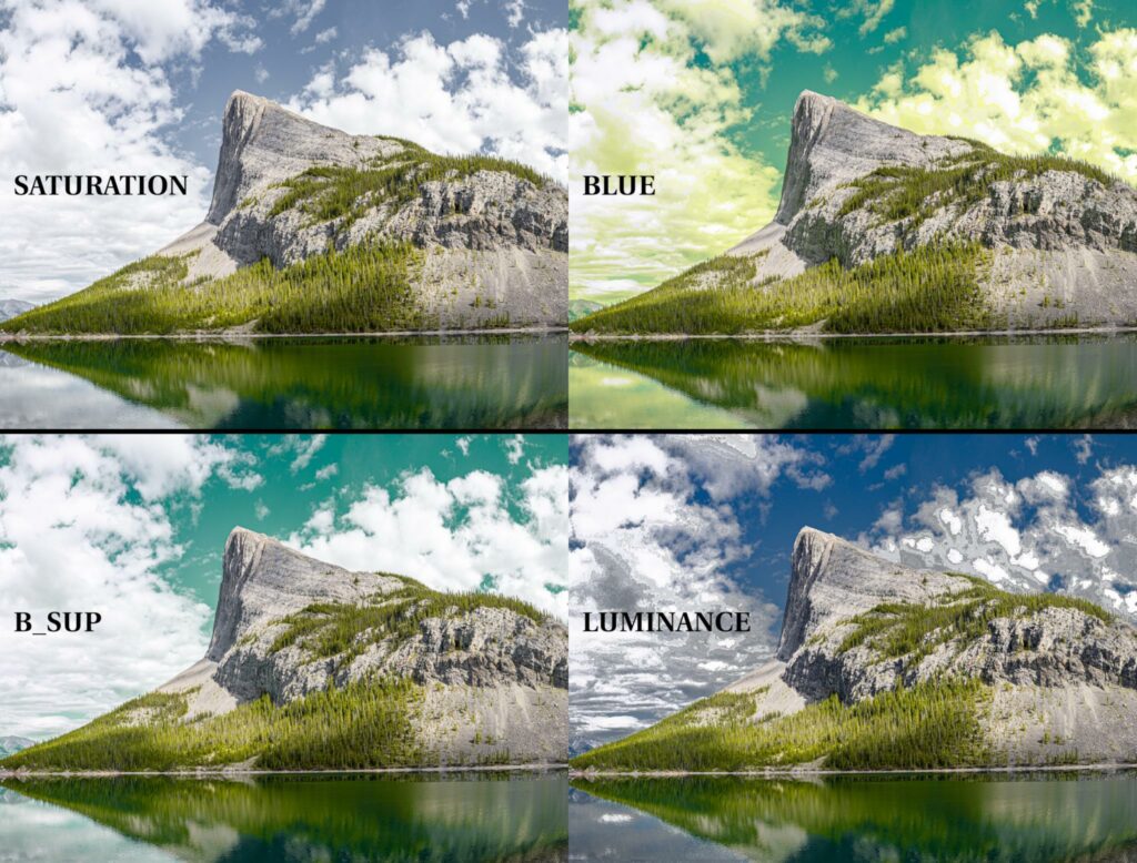
To sum it up we should look at some real footage. Let’s say we are working on the sky.
As we’ve seen, the saturation operation will give us a nice, weighted solution to decrease the chroma – by balancing all 3 channels. This gives us a nice, natural response.
If we isolate the blue channel on the other hand, we will not accomplish a reduction in saturation, but rather a shift in colors. We’ve learned that this is a simple multiplication of the blue channel – so as if you’re using a multiply or gain of the grade node. That means decreasing blue leads to introducing more yellow or orange. Since we’re not involving the other channels, it can make our image look less believable quite quickly if we dial it in too harshly.
If you look at this way: By tweaking R, G and B separately on a Grade node, we’re already splitting up the image into 3 components – with the HueCorrect node, you could now go in and for one single channel only tweak one specific hue. So that’s cutting your margin down even further.
Now you can imagine why it can look quite graphic real quick. But it’s definitely great for very specific or subtle treatments. And of course, you can always smoothen out your curve in order to avoid harsh transitions.
Blue suppression on the other hand takes the other channels into account, so the result is less extreme. It only includes the other channels to produce new values for the channel we are tweaking it for though – in this case blue – but it doesn’t affect the other channels itself.
This way you can focus on a very dominant hue as we would find in blue and green screens and counteract with a color shift – without being too aggressive on other channels.
But keep in mind that you will be bound for this specific despill algorithm. If you want to be more flexible you’ll definitely need to use some dedicated despill setups or gizmos.
Luminance uses a multiplication for all 3 channels – but, it can also break real quick, since hue values sometimes change a lot from pixel to pixel or are not that obvious in very bright areas and you can end up with some pretty nasty edges if you push it too much.
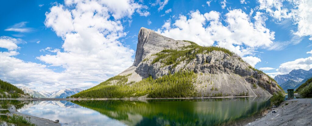
Here is another good example:
If we want to reduce the warm orange-yellow tones in those trees, we could use a multiplication on the R channel, but it will also adjust the areas in the background underneath the massive rocks.
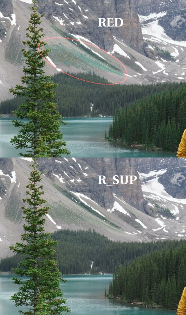
The despill algorithm preserves this area, since it’s checking if red contributes the brightest pixel values here – which is not the case, so it stays untouched.
So always make sure to stop for a second, be aware of what you want or need to do and what the underlying operation does mathematically – and then you will know what it can do for you.
You can download the Nuke script that I set up for the deconstruction of the HueCorrect node here: Deconstruct_HueCorrect